If you have ever conducted a survey, you have probably noticed that the devil is in the detail. Errors, distortions, and biases can happen throughout the process—from designing the questionnaire to collecting responses and analyzing results.
A common objection to surveys is regarding the representativeness of results. Maybe you’ve heard some of these sentences before:
- “Will the people we want to hear from actually respond to this survey?”
- “Are these results fully reflecting our audience?”
- “It seems like only a very specific group of our audience has taken this survey.”
And yes, your sample of survey respondents probably never accurately reflects the entire group of people you want to draw conclusions about. First, let’s look at why this is the case. Second, let’s have a look at weighted survey analysis and see how it can mitigate the problem to some extent.
Why your sample is probably biased
Here’s a cartoon I like that illustrates the point in question quite well. Something is wrong with the sample of survey respondents shown in the chart:
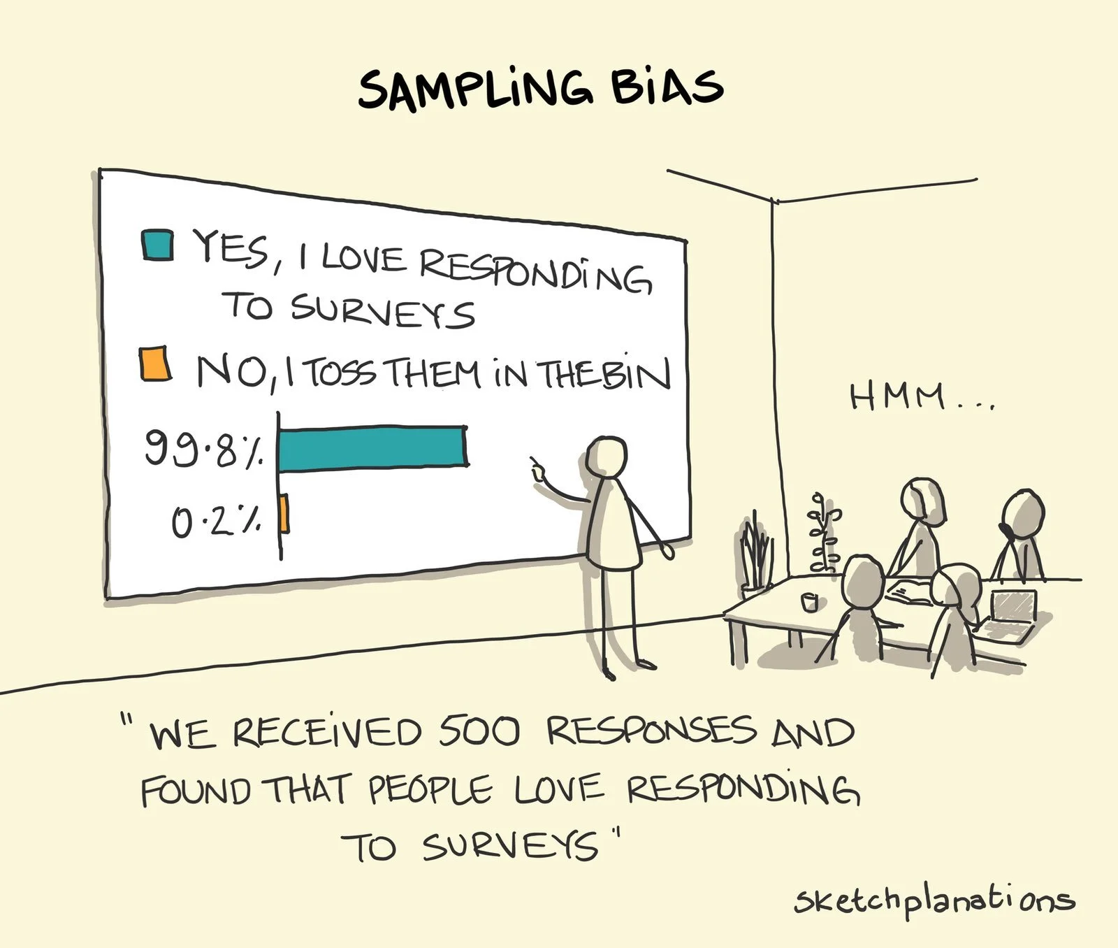
Cartoon by sketchplanations
Two biases come to mind looking at the cartoon:
- The people who end up taking your survey might differ quite a lot from those who don’t. (For example, they don’t hate surveys.) If you’re unlucky, your respondents differ from non-respondents in ways that distort your results. This is called non-response bias.
- The people you invited to the survey might not have been representative of your audience in the first place. This can happen if you (1) only invite a subgroup of your target population to the survey (i.e., a sample, which is almost always the case) and (2) some people are more likely than others to be included in that subgroup. It’s called sampling bias.
Both biases lead to the same outcome: your sample will be different from the larger group you want to draw conclusions about (i.e., the population).
What can you do about this? First, improve the survey invitation process. Aim to invite a non-biased group of people to the survey (e.g., with a random sample) and set up the conditions so that a non-biased group of people responds to it (e.g., by reducing barriers to respond). However, response behavior is hard to influence directly.
Survey weighting can also help in the case of a biased sample when responses are already collected. It’s a helpful statistical tool, even if it can’t compensate for a biased data collection setup.
How can a weighted analysis help?
In a nutshell, weighted survey analysis amplifies the responses from under-represented respondents and dampens the responses from over-represented respondents.
The overall idea is to assign each respondent a weight that influences their impact on the statistics you calculate. With these weights, you can adjust the frequency distributions for certain variables in our sample in such a way that they resemble those of the population. The variables used for comparing sample and population distributions are the adjustment variables.
Here’s an example. If age group is an adjustment variable and younger people are over-represented in your sample, we might want to assign weights to our survey respondents in such a way that the few older respondents in your sample get a higher weight and a higher impact on the statistics we calculate.
To sum up the overall intuition for survey weighting:
- Respondents who are over-represented in your sample will get a lower weight in your analysis so that their impact on the statistics you’re calculating gets reduced.
- Respondents who are under-represented in your sample will get a higher weight in your analysis so that their impact on the statistics you’re calculating gets amplified.
Which weighting approach should you use?
There are many different weighting approaches with different levels of complexity. This report by Pew Research gives a good overview of the topic and some initial takeaways. The following stood out to me:
“When it comes to accuracy, choosing the right variables for weighting is more important than choosing the right statistical method.”
“The most basic weighting method (raking) performs nearly as well as more elaborate techniques based on matching.”
“Even the most effective adjustment procedures were unable to remove most of the bias.”
— Pew Research (2018): For Weighting Online Opt-In Samples, What Matters Most?
Based on these insights, a pragmatic approach for survey weighting can be to go with a simple raking algorithm and invest a good amount of time in the discussion and selection of adjustment variables. Also, it seems important to lower expectations about weighted analyses because they won’t get rid of all the bias.
For selecting the adjustment variables, I used the following criteria as a starting point:
- There needs to be a reason or rationale for why the adjustment variable might influence the results. According to Pew Research, variables related to the survey topic often work better for weighting than basic demographics.
- You need to know the adjustment variable’s population frequencies. For example, if you want to use your responding customers’ spending as a weighting variable, you need to know the spending within your entire customer base (which, in this example, you probably do).
- Adjustment variables need to be categorical for raking.
For market and user research surveys so far, I have seen engagement-related and behavioral variables work best for weighting. But I’m still learning what works best in which situation.
How to compute survey weights in R
My suggested basic implementation for survey weighting in R makes use of the anesrake package. It’s meant to be a starting point, and you probably need to adapt or extend it for your use case.
Step 0: Load required packages
Let’s start by loading the required packages. These two are all we need for now:
library(tidyverse)
library(anesrake)
Step 1: Make sure all adjustment variables are in the survey dataset
Sometimes, the adjustment variables are already in the survey dataset because they were generated with survey questions. In other cases, you might want to conduct weighting based on variables from your customer database, in which case they need to be matched to the survey responses—this has to be taken into account during data collection.
Step 2: Check for missing data in the adjustment variables
The anesrake algorithm can’t work with missing data in the adjustment variables. Based on your specific use case, you need to decide on a way to remove or impute missing values. Some options are outlined in this freeCodeCamp article.
You can start by counting the missing values for each variable of your dataset and go from there:
map_df(survey_data, ~sum(is.na(.x)))Step 3: Transform your survey data to work with anesrake
For anesrake to work correctly, your data needs to be a base data frame and all adjustment variables need to be factors. You can handle these transformations like this:
survey_data <- as.data.frame(survey_data)

survey_data <- survey_data %>%
  mutate(across(c(weighting_var_1, weighting_var2), as.factor))
Step 4: Add an ID variable to your survey dataset, if there isn’t one already
Your dataset needs an ID column that uniquely identifies responses for later matching with the computed weights. If you don’t have one already, create a simple ID based on row number:
survey_data <- survey_data %>%
  mutate(id = 1:nrow(survey_data))
Step 5: Enter the population frequencies for the adjustment variables
Anesrake needs to know the adjustment variables’ population distributions to compute weights. These will be stored as a list of named vectors. Assuming our adjustment variables are age group and some type of product engagement, the population distributions need to be in the following format:
targets <- list(
  age_group = c(
    "18-24" = 0.31,
    "25-34" = 0.34,
    "35-44" = 0.18,
    "45-55" = 0.11,
    "above 55" = 0.05
  ),
  engagement = c(
    "low" = 0.15,
    "medium" = 0.62,
    "high" = 0.23
  )
)
Step 6: Run the raking algorithm
We’re ready to run the actual raking procedure.
raking_result <- anesrake(
  inputter = targets,
  dataframe = survey_data,
  caseid = survey_data$id
)
Extract the weights like this.
weights <- tibble(
  id = names(raking_result$weightvec),
  weight = raking_result$weightvec
)
It’s also worth exploring the anesrake list object (here: raking_result) a bit further. For example, the element “varsused” will tell you which of your specified adjustment variables have actually been used for weighting. Your adjustment variables might not have been used if their sample distributions didn’t differ much from the population distribution. By default, anesrake only includes adjustment variables when there is a discrepancy of more than 5%. You can change this default with the pctlim argument.
Step 7: Add the weights to the survey dataset
Add the computed weights to the survey dataset, joining by ID. Note that the ID column in the weights data frame is in character format because it was derived from the names attribute of the raking_results$weightvec vector. To make the join work, I converted the ID column in the survey dataset to character format as well.
survey_data <- survey_data %>%
  mutate(id = as.character(id)) %>%
  left_join(weights, by = "id")
How to do weighted analyses in R
To make use of the brand-new weight variable, we need to use weighted statistics from now on. There are many different functions available for this, the following of which I have used most often:
stats::weighted.mean()— Calculate a weighted mean.weights::wpct()— Calculate a weighted frequency table with percentages.weights::wtd.cors()— Calculate weighted correlations. If you want standard errors and a test of significance as well, useweights::wtd.cor()instead.Hmisc::wtd.var()— Calculate a weighted variance. If you’re interested in the weighted standard deviation, just take the square root of this one.Hmisc::wtd.quantile()— Calculate weighted quantiles.
These statistics are a good starting point for many analyses. Make sure to always specify the weight variable in the function calls. Some of these functions work without a weight variable, which means you won’t see an error if you forget to include it.
Conclusion
Survey weighting can lead to more representative statistics when working with a biased sample. It’s straightforward to implement in R when using a basic raking algorithm like anesrake.
I have yet to encounter a dataset and scenario where the weighted analysis leads to completely different results and takeaways. Often, the differences seem to be rather subtle.
In any case, considering a weighted analysis seems like a good mental exercise because it forces you to consider the ways in which a sample might be biased.
References